Why Cost Volume Construction Can Be a Non-Trivial Yet Interesting Problem in Transformer-Based Models?
A technical post reflecting our work in leveraging Transformer architecture for reconstruction
Introduction
Since the introduction of the Transformer architecture in 2017 by Vaswani et al., it has gained increasing attention from its original domain Natural Language Processing (NLP) to Computer Vision (CV). Because of its impressive learning capability, Transformer-based methods have achieved state-of-the-art (SOTA) results in various tasks. For many research endeavors nowadays, the first thing on the list is to find a way to tokenize structured data representation into unstructured ones that Transformer can process since it only inherently takes a sequence of tokens. This blog won’t go into much detail about the tokenization process as it’s still an open question about what’s the most effective way to preprocess and tokenize a certain data representation, from my perspective. I’d like to talk about in my recent research work ODTFormer, how we formulate the problem of 3D computer vision, specifically depth estimation and reconstruction, into Transformer-acceptable form with an intuitive yet effective design.
Cost Volume
Cost volume in computer vision refers to the volumetric representation of cost or similarity of matching pixel windows or features between two or more images. Why is it essential? Because for stereo (two images or views) and multi-view stereo (more than two views) depth estimation, in the simplest case with two rectified images (in a nutshell, the corresponding points on two images of a 3D point should have the same y-coordinate meaning no vertical shift), the epipolar geometry tells us that the depth (Z) of a certain 3D point, visible on both images, can be calculated as \(Z = B * f / disparity\) as shown in the figure below, where \(B\) refers to the baseline (distance between two cameras), \(f\) is the camera focal length as part of the camera intrinsic and \(disparity\) is the shift in the x-coordinate of the corresponding points’ coordinates on the two images.
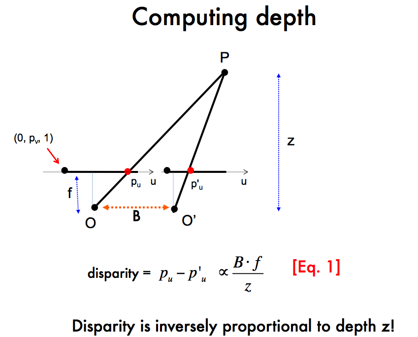
So theoretically, if we can get accurate disparity measurements, depth estimation can be straightforward. But in real-world applications, several detrimental factors exist, like imperfect camera parameters, rectification or lens distortions, etc., one dominant issue is that finding accurate pixel correspondences between the two images can be challenging!
Then comes the technique used by most of the depth estimation methods nowadays.
Learning-Based Cost Volume Construction
Let’s simplify the problem to only about stereo reconstruction that only have two images of different views. Conventionally, the cost volume is constructed by first extracting feature maps using image backbone and then given a predefined depth range, a disparity range of interest can be calculated through reversing the equation above. At each disparity level, feature maps can be overlapped or interlaced on each other, then processed by 2D or 3D convolution blocks to get the matching costs where the values will form distribution to the cost/similarity of certain pixel under this disparity level. Eventually, the matching costs from all disparity levels will be concatenated to form the cost volume (if the size of feature map is \(H \times W\), it becomes \(D \times H \times W\) where D is the number of disparity levels) and can be processed by another 3D convolution block to get the final volume.
Reflecting on this process, it’s an exhaustive search method that iterates through all possible disparities where some camera parameters and training data-specific settings are inevitably being hardcoded into the model during the training process, leading to issues for model generalizability and computation efficiency. But because of the nature of convolution architecture being good at handling structured data representations, such approach shows impressive performances in depth estimation and reconstruction.
Cost Volume meets Transformer
However, the cost volume construction method has some fatal weaknesses when trying to combine it with a Transformer-based architecture. First of all, although there’s already a quite mature pipeline of how Transformer can be used to process 2D image data pioneered by Vision Transformer (ViT) through splitting an image into uniform-sized patches and extracting token features for each patch. But the cost volume requires adding dimension to the data which needs to consider a lot more extra factors, such as, what’s the meaning of information carried by the dimension, do we process it as a whole or partition it into more fine-grained features. Moreover, because of the quadratic growth in the computational complexity of the Attention mechanism - the core of Transformer architecture - the effect of resultant tokens from tokenizing the entire 3D volume to the performance of Attention operation cannot be ignored.
Is it simply infeasible to adapt the concept of cost volume into Transformer-based models?
Voxel Occupancy Detection
Voxel occupancy detection is a subtask of reconstruction in 3D computer vision, the term Occupancy Grid is defined as a data structure that partition a 3D space into uniform sized voxel cubes and each cube can be marked as either occupied or unoccupied. The occupancy grid is a common data structure being leveraged in robotic navigation and autonomous driving systems to improve computation efficiency and data interpretability. Previous navigation works using voxel occupancy detection usually lie in two settings - Stereo (two font cameras) and Bird’s-Eye View (BEV, six surrounding cameras).
Almost all prior works under the stereo setting use the cost volume construction method since it’s the most straightforward application as we discussed before, the images can be easily be rectified because of the nature of stereo camera setup and it has been proven effective by numerous stereo depth estimation works. What about BEV settings?
Adapting cost volume construction to occupancy detection in BEV turns out to be non-trivial given the fact that there are certainly more than horizontal shifts in some camera pairs under BEV settings and how to effectively construct cost volume with more than two views remains an open question under many aspects. Therefore, most of the BEV detection works use Transformer-based methods to tackle this problem. One of the most influential work in BEV is BEVFormer uses a type of spatial attention called Multiscale Deformable Attention mechanism.
Multiscale Deformable Attention (MDA) Mechanism
The Multiscale Deformable Attention (MDA) mechanism is first introduced by Zhu et al. in Deformable DETR for object detection in 2D images. It consists of five steps: first initialize queries from spatial locations on the 2D image, then the queries will be fed to a Learnable Offset Sampler which generates a set of predefined number of offsets for each query per feature map scale. For each query, the offsets will be applied to its associated spatial location on each feature map, producing the set of sampling locations. Finally, the set of feature tokens can be obtained from the feature maps through grid sampling using the sampling locations and the query will be attending the set of selected tokens.
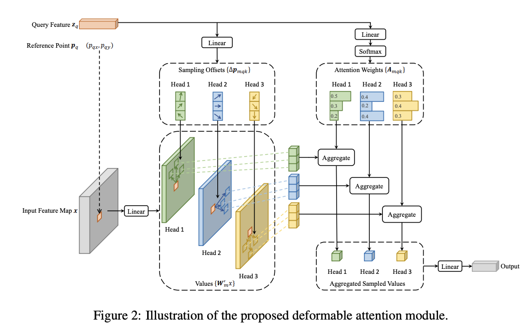
The Multiscale Deformable Attention mechanism excels at both task performance and computational efficiency because it’s a type of guided Attention, instead of vanilla Attention which simply attends to all feature tokens, the Deformable Attention only attends to tokens that are considered relevant. In Computer Vision tasks, attending to all tokens can inevitably introduce noise and unwanted information from irrelevant tokens. The sampling process also greatly reduces the computational complexity caused by the quadratic growth in the Attention mechanism as mentioned earlier.
MDA in BEV Occupancy Detection
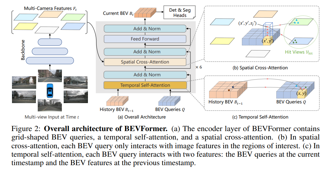
Since it’s not easy to directly adapt cost volume construction into BEV setups given various constraints, this is where MDA comes in handy. BEVFormer introduced a pipeline using MDA which is referenced by lots of BEV works afterward. As the camera intrinsics and poses are known in these tasks, they can be used to project coordinates in 3D space onto 2D images. Therefore, the Spatial Cross-Attention in BEVFormer works as follows - Given the multi-scale feature maps extracted from BEV images, the queries for voxels within the occupancy grid are initialized using the 3D center coordinates of the voxels and the corresponding 2D coordinates for each view are obtained through direct projection using camera parameters, and then the queries go through the same MDA process to produce query outputs per view. Eventually, the multi-view outputs are aggregated through averaging the outputs from views that the 3D query coordinates fall into and producing the final feature of each voxel.
Stereo Occupancy Detection meets MDA
In our recent work ODTFormer, we aim to solve the stereo occupancy detection problem with a Transformer-based architecture. However, after extensive experiments of directly using the MDA following BEVFormer’s manner, the model always fails to outperform the SOTA method StereoVoxelNet, uses cost volume construction and Convolutions, in stereo occupancy detection by a great margin. Only when we modify MDA to process 3D data and attending to a conventional cost volume shows some improvements in metric measurements while still unable to get close to StereoVoxelNet.
These phenomena makes us realize that matching cost could be an essential inductive bias in 3D reconstruction, but with the obstruction mentioned above, how to effectively combine cost volume construction with Attention or Transformer models?
Deformable Matching Cost Block
In ODTFormer, we discovered a simple yet surprisingly effective design that can introduce the matching costs as inductive bias into the Transformer-based model while differing the conventional cost volume construction, called Deformable Matching Cost (DMC) Block.
The changes in the DMC operation compared to the usage of DMA in BEVFormer are as follows - instead of carrying out the feature sampling process in 2D space entirely, we use the 3D voxel center coordinates with a set of 3D sampling offsets constrained by the target voxel size to get 3D sampling locations, then locations are projected to 2D corresponding points and get the features. Moreover, to further enforce feature correspondences, we don’t use different sampling locations per scale, but directly scale the sampling coordinates so that they always correspond to the same set of 3D points on different scales. Furthermore, we use two separate Multi-Layer Perceptrons (MLP) to first concatenate and merge the feature channels from the tokens extracted from two views corresponding to the same 3D point per scale, the second MLP is used to concatenate and merge the output tokens across multiple scales to get the final set of tokens that contain multi-view and multi-scale matching cost information.
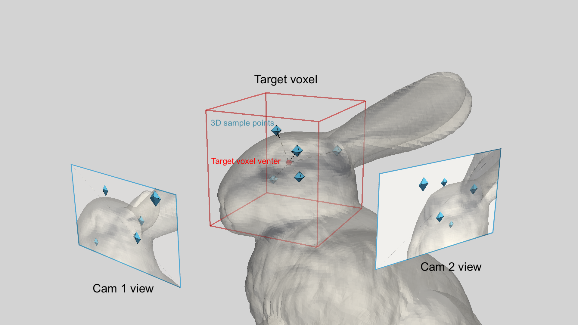
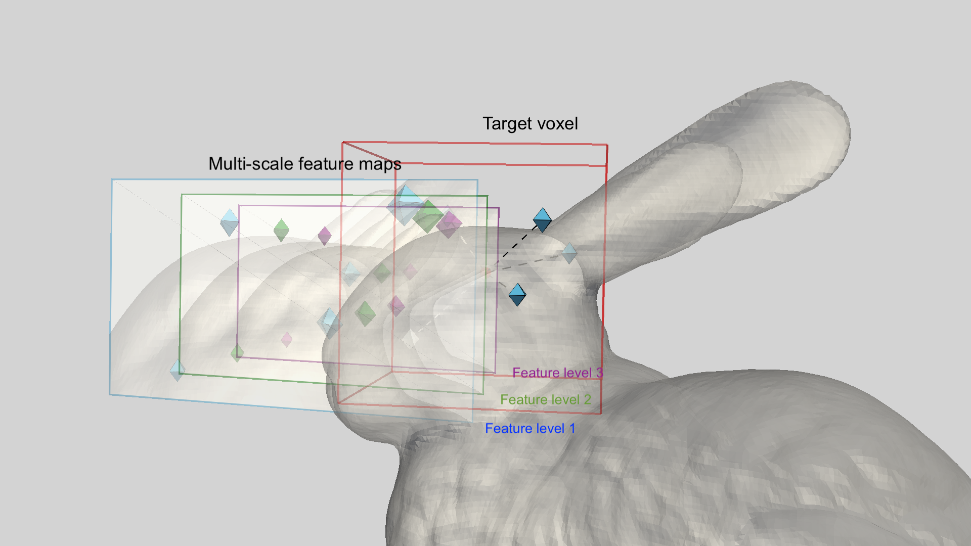
Finally, the queries attend to the extracted matching cost tokens to produce the voxel features as a cost volume for each voxels that we are interested in and are further decoded into voxel occupancy grids.
The model metric evaluations show that our approach outperforms StereoVoxelNet by a great margin with minimal increase in computational complexity, and although the coarse-grained voxel size we use for sampling is \(3m\), our model still achieves the best accuracy after decoding into fine-grained voxel size of \(0.375m\). This observation further supports that matching cost is an essential factor as inductive bias that can greatly boost reconstruction model performances and the effectiveness of our DMC block design. The best part of it is that the theoretical applications of DMC block can be extended to multi-views with minimal modifications.
Conclusion
It’s fascinating to dive deep into the topic of how the technique of cost volume construction can be reformulated to fit of a Transformer-based model, but what lies more within such research endeavor is that if we can correctly find the sweet point of how to reformulate the problem representation of the model considering certain invariants. Simple yet intuitive designs can also greatly boost the model performance without affecting computational efficiency which can be useful for improving model robustness and generalizability across different domains and settings, as well as its affordability on edge devices.